The Journal of Physical Chemistry C
DOI: 10.1021/acs.jpcc.8b07804


from Journals via hj on Inoreader http://bit.ly/2D7VSrg


The aim of this paper is to examine the relationship between CO2 emissions and its possible determinants and their direction of causality for Pakistan over the period of 1972 to 2017. The survey of literature guides us that the most frequently discussed factors are real GDP per capita, energy consumption, urbanization, trade openness, and financial development. Testing of environmental Kuznets curve (EKC) hypothesis is the most common in environment literature so we also incorporated the real GDP per capita squared term in the model. Autoregressive distributed lag (ARDL) bound testing approach to cointegration with structural break and error correction method (ECM) are applied to the selected time series to investigate the long-run relationship between CO2 emissions and real GDP per capita, real GDP per capita squared term, energy consumption, urbanization, trade openness, and financial development. The empirical evidence confirms the cointegration among the variables and EKC holds for Pakistan support H1 of the study, which though contradictory to the previous studies conducted on Pakistan but all of previous work faces the exclusion bias and their findings were skewed. The findings also suggest that energy consumption and urbanization have a positive effect on CO2 emissions, supporting H2 and H3. However, H4 and H5 rejected as trade openness and financial development found positively significant. Moreover, bidirectional Granger causality was exists only between CO2 emissions and trade openness. The findings suggests that Pakistan need to settle the economic agenda of the nation through the resolution of economic controversies, energy mix need to tilt toward clean and renewable energy, and rural-urban migration need to manage for better air, water, and living.


The linkage between financial development and energy consumption is widely investigated in the literature. However, the non-linear relationship between financial development and energy demand is still under debate. Therefore, this study aims to examine the non-linear relationship between financial development, economic growth, and energy consumption in OECD countries. The study uses the Driscoll–Kraay standard errors panel regression model for spanning from 1980 to 2016. The empirical findings indicate that an inverted U-shape relationship exists between financial development and energy consumption as well as between economic growth and energy consumption. Moreover, the feedback hypothesis is found between financial development and energy use. Additionally, income and energy use granger cause each other. The innovative findings contribute to extant literature, which is of special interest to the country's policymakers regarding energy efficiency.
Few detailed, individual-focused studies have researched the added effect of temperature on cardiovascular disease (CVD), particularly in China. Moreover, no prior studies have explored the exposure-response relationship among all populations and different sub-sociodemographic groups. A distributed lag nonlinear model (DLNM) was applied to evaluate the adverse health effects of temperature on CVD mortality for all populations and different sub-sociodemographic groups (by age, sex, educational level, living arrangement, and occupation) in Beijing. Based on the exposure-response relationships, firstly, we proposed a new model (COCKTAIL, Code Of Climate Key To An Ill) for revealing the split-and-merge relationships of the temperature-CVD mortality curve. This method could be used to apply the CVD deaths in a studied area to forecast the exposure-response relationships in the same area in the future. Secondly, this is the most detailed study to analyze the relationship between temperature and CVD mortality for different subgroups among the existing researches for developed and developing countries. We found that the cold temperature (at − 14 °C) was the risk factor for people with low socioeconomic status, especially for single people (including unmarried, divorced, and widowed), for indoor workers, and for people with low education, compared with the minimum mortality temperature, with a cumulative increase of 3.9 (80%CI, 2.9–5.4), 3.8 (80%CI, 2.8–5.1), and 4.5 (80%CI, 3.1–6.3) times respectively. Meanwhile, the hot temperature (at 35 °C) was the risk factor for CVD death, with a cumulative increase of 2.6 (80%CI, 2.0–3.4) for females, and 3.1 (80%CI, 2.4–4.2) for single people. The varying CVD vulnerability in terms of CVD mortality among various groups may assist governments in preparing health resources and taking measures to prevent or reduce temperature-related deaths.
We are finally at the most crucial part of the modeling process: proving if the damned thing works.
Not "works" in the sense that we get good unobservable parameter estimates, but works in the sense that the model makes useful, skillful predictions. No model should ever be released, by any researcher, until it has been verified at least using old data, and preferably using never-before-seen-or-used-in-any-way data. I'll later have a paper on this subject, but I go on and on about it in this award-eligible book.
We're going to use the Boston Housing data available in the mlbench package in R.
  install.packages("mlbench")
  require(mlbench)
  data(BostonHousing)
  ?BostonHousing
The last line of code will explain the dataset, which is 500-some observations of median housing prices (in $1,000s), from the 1970 Census, in different Boston neighborhoods. The key measure was nox, atmospheric "nitric oxides concentration (parts per 10 million)", which we will take was measured without error. Which is not likely. Meaning that if we could take into account whatever uncertainty in the measure exists, we should use it, and the results below would be even less certain.
The idea was that high nox concentrations would be associated with lower prices, where "associated" was used as a causal word. To keep the example simple yet informative, we only use some of the measures: crim, per capita crime rate by town; chas, Charles River border indicator; rm, average number of rooms per dwelling; age, proportion of owner-occupied units built prior to 1940; dis, weighted distances to five Boston employment centres; tax, full-value property-tax rate; and b, a function of the proportion of blacks by town.
The ordinary regression gives this ANOVA table:
fit = glm(medv ~ crim + chas + nox + rm + age + dis + tax + b, data=BostonHousing) summary(fit) Estimate Std. Error t value Pr(>|t|) (Intercept) -11.035298 4.193677 -2.631 0.00877 crim -0.110783 0.036748 -3.015 0.00270 chas1 4.043991 1.010563 4.002 7.25e-05 nox -11.068707 4.145901 -2.670 0.00784 rm 7.484931 0.381730 19.608 Look at all those excitingly wee p-values. Glorious, no? No. We'll soon see they lead to bitter disappointment.
Let's now fit the Bayesian version of the same regression, using defaults on the priors as we've been doing. We'll fit two models: one with nox, one without.
  fit.s = stan_glm (medv ~ crim + chas + nox + rm + age + dis + tax + b,data=BostonHousing)
  fit.s.n = stan_glm (medv ~ crim + chas + rm + age + dis + tax + b,data=BostonHousing)
We could look at the summaries of these models, and you should, but they would only give information about the posterior parameter distributions. Since we're using numerical approximations (MCMC methods) to give answers, we should see if the algorithms are working. They are. We could do better by tuning the approximation (larger resamples), but the defaults are close enough for us here.
So how do we check if the model works?
We have to ask a question that is pertinent to a decision we would make using it. The third quartile observed housing price was $35,000. What is the predicted probability prices would be higher than that given different levels of nox for data not yet observed? The answer for old data can be had by just looking. Why this question? Why not? If you don't like it, change it!
In order to answer our question, we also have to specify values for crim, chas, and all the other measures we chose to put into the model. I picked median observed values for all. If you have other questions or other values you like, try them!
Let's look at the predictions of housing price for future varying levels of nox: I used a sequence from the minimum to maximum observed values, with all other measures at their medians.
nnox = seq(min(BostonHousing$nox),max(BostonHousing$nox),by=.01) s = length(nnox) newdata = data.frame(crim = rep(median(BostonHousing$crim),s) , chas = rep("0",s) , nox = nnox , rm = rep(median(BostonHousing$rm),s) , age = rep(median(BostonHousing$age),s) , dis = rep(median(BostonHousing$dis),s) , tax = rep(median(BostonHousing$tax),s) , b = rep(median(BostonHousing$b),s) ) p.s.n = posterior_predict(fit.s,newdata) p.s.non = posterior_predict(fit.s.n,newdata) We built predictions many times before, so if you've forgotten the structure of this code, review! Now let's see what that looks like, in a relevance plot:
plot(nnox,colMeans(p.s.n>35), type='l', lwd =3, xlab='nox (ppm)', ylab='Pr(Price > $35,000 | XDM)') lines(nnox,colMeans(p.s.non>35), lwd = 2, col=4) grid() legend('topright',c('With nox','No nox'), col=c(1,4), lty=1, lwd=3, bty='n') 
The predictive probability of high housing prices goes from about 4% with the lowest levels of nox, to something near 0% at the maximum nox values. The predictive probability in the model without nox is about 1.8% on average. The original p-value for nox was 0.008, which all would take as evidence of strong effect. Yet for this question the probability changes are quite small. Are these differences (a +/- 2% swing) in probability enough to make a difference to a decision maker? There is no single answer to that question. It depends on the decision maker. And there would still not be an answer until it was certain the other measures were making a difference. I'll leave that as homework.
We need this helper function, which is a simple adaptation of the original, which I don't love. If you'd rather use the original, have a ball.
ecdf Now this is a fun little plot. It shows the probability prediction of Y for every old observed X, supposing that old X were new. This assumes my version of ecdf.
# the old data is reused as if it were new p.s = posterior_predict(fit.s) P = ecdf(p.s[,1]) plot(P$vals, P$ecdf, type='l',xlim=c(-20,60), xlab="Price = s", ylab="Pr(Price 
Price (s) in on the x-axis, and the probability of future prices less than s, given the old data and M(odel), are on the y-axis. A dotted red line at $0 is shown. Now we know based on external knowledge to M that it is impossible prices can be less than $0. Yet the model far too often gives positive probabilities for impossible prices. The worst prediction is about a 65% chance for prices less than $0. You remember we call this probability leakage.
So right now we have good evidence this model has tremendous failure points. It is not a good model! And we never would have noticed had we not examined the model in its predictive form---and we also remember all models have a predictive form: even if you don't want to use that form, it's there. What we should do at this point is change the model to remove the leakage (and surely you recall we know how to do that: review!). But we won't: we'll keep it and see how the rest of the model verifies.
Let's look at four predictions, picking four old X, because the all-predictions plot is too busy. And on this we'll over-plot the ECDF of the observations, which are, of course, just step functions.
par(mfrow=c(2,2)) for (j in base::sample(1:nrow(BostonHousing),4)){ P = ecdf(p.s[,j]) plot(P$vals, P$ecdf, type='l',xlim=c(-20,60), xlab="Price = s", ylab="Pr(Price From this plot we have the idea that the closer the ECDF of the prediction is to the ECDF of the observation, the better the model does. This is a good idea, indeed, a great one. It leads to the idea of a score that measures this distance.
One such, and very well investigated, score is the continuous ranked probability score, or CRPS. It is not the only one, just the one we'll use today.
Let F_i(s) = Pr( Y < s | X_i D_n M), i.e. a probabilistic prediction of our model for (past) measure X_i (which can be old or new; the D_n is the old data, as we have been writing). Here we let s vary, so that the forecast or prediction is a function of s, but s could be fixed, too. Let Y_i be the i-th observed value of Y. Then
CRPS(F,Y) = sum_i ( F_i - I( s ≥ Y_i ) )^2,
where I() is the indicator function. If s is fixed and Y dichotomous, CRPS is called the Brier score. We can look at CRPS for each i, or averaged over the set. There are various ways to calculate CRPS, depending on the model assumed. Here we'll just use straight-up numerical approximation.
Why not use RMSE or MAD or R^2? Because those scores are not proper. I'll write elsewhere of this, but the idea is those scores throw away information, because they first have to compress the probability (and all our predictions are probabilities) into a point, thus they remove information in the prediction, leading to suboptimal scores. Proper scores have a large literature behind them---and you already know which award-eligible book writes about them!
Let's calculate, for both models with and without nox, the CRPS for each old observation.
crps = NA crps.n = NA k = 0 for (j in 1:nrow(BostonHousing)){ k = k + 1 sf=stepfun(BostonHousing$medv[j],c(0,1)) P = ecdf(p.s[,j]) crps[k] = sum((P$ecdf - sf(P$vals))^2)/length(P$ecdf) sf=stepfun(BostonHousing$medv[j],c(0,1)) P = ecdf(p.s.n[,j]) crps.n[k] = sum((P$ecdf - sf(P$vals))^2)/length(P$ecdf) } plot(BostonHousing$medv,crps, xlab="Price ($1,000s)", ylab="CRPS (with nox)",ylim=c(0,.35)) The stepfun creates a function which we use to compute the value of the ECDF of the observed price, which we need in our approximation of CRPS. Note, too, it uses the already computed posterior predictions, p.s. The crps is for the nox model; and crps.n is for the non-nox model. The plot is of the individual CRPS at the values of prices.

See that "floor" in the CRPS values? Looks like CRPS can go so low, but no lower. This turns out to be true. Given a model form, we can calculate an expected CRPS, and then bust up that expectation into pieces, each representing part of the score. One part is the inherent variability of the Y itself. Meaning, given a model, we have to accept the model will only be so good, that uncertainty will remain. There is much more to this, but we'll delay discussion for another day.
We could also do this:
plot(crps.n,crps, ylab="CRPS (with nox)", xlab="CRPS (no nox)") abline(0,1) I won't show it, because it's hard to see, by eye, whether the nox model is doing better. But you can look on your own.
Enter the idea of skill---which was another of Fisher's inventions. Again, you know where you can read about it.
Skill scores K have the form:
K(F,G,Y) = ( S(G,Y) - S(F,Y) ) / S(G,Y),
for some score function S(.,Y) (like CRPS), where F is the prediction from what is thought to be the superior or more complex model and G the prediction from the inferior. Skill is always relative. Since the minimum best score is S(F,Y)=0, and given the normalization, a perfect skill score has K = 1. Skill exists if and only if K >0, else it is absent. Skill like proper scores can be computed as an average or over individual points.
Models without skill should not be used!
Why not? Because the simpler model beats them! If you don't like CRPS, then you should, always should, use the score that reflects the cost-loss of the decisions you will make using the model. As always, a model may be useful to one man and useless to another.
Here is the skill plot:
plot(BostonHousing$nox,(crps.n-crps)/crps.n, ylab="Skill", xlab="nox") abline(h=0,lty=2,col=2) 
Everything below 0 are times when the non-nox model did better.
The overall average skill score was K = -0.011, indicating the more complicated model (with nox) does not have skill over the less complicated model. This means, as described above, that if the CRPS represents the actual cost-loss score of a decision maker using this model, the prediction is that in future data, the simpler model will outperform the more complex one.
We don't actually know how the model will perform on future data, we can only guess. So that model scores on old data are themselves predictions of future performance. How good they are is an open research question; i.e. nobody knows.
Whether this insufficiency in the model is due to probability leakage, or that the CRPS is not the best score in this situation, remain to be seen.
We have thus moved from delightful results as indicated by p-values, to more sobering results when testing the model against reality---where we also recall this is only a guess of how the model will actually perform on future data: nox is not useful. Since the possibility for over-fitting is always with us, it is the case that future skill measures would likely be worse than those seen in the old data.
Most of this post is extracted from an upcoming (already accepted) paper, which will be posted when it is published. This post is only a bare sketch.
The most recent mass media contribution to the canon of climate alarmism referenced a study claiming that "climate change" (i.e., human-caused deep ocean warming) was responsible for the Amundsen Sea's (West Antarctica) "rapid melting" of the Thwaites Glacier.
A few months ago, however, scientists (Jenkins et al., 2018) reported that the Amundsen Sea sector – where Thwaites glacier is located – has been in a cooling phase since 2009-'11.
Furthermore, the ocean in this region warms and cools in accordance with decadal-scale cycles. Consequently, the authors conclude that the "accelerated mass loss from the Amundsen Sea sector of the [West Antarctic Ice Sheet, WAIS] has not resulted from progressive ocean warming or unstable ice retreat."
This would appear to contradict the claim that rapidly and linearly rising anthropogenic CO2 emissions are what lies behind the ocean warming and/or ice sheet melt for this region.
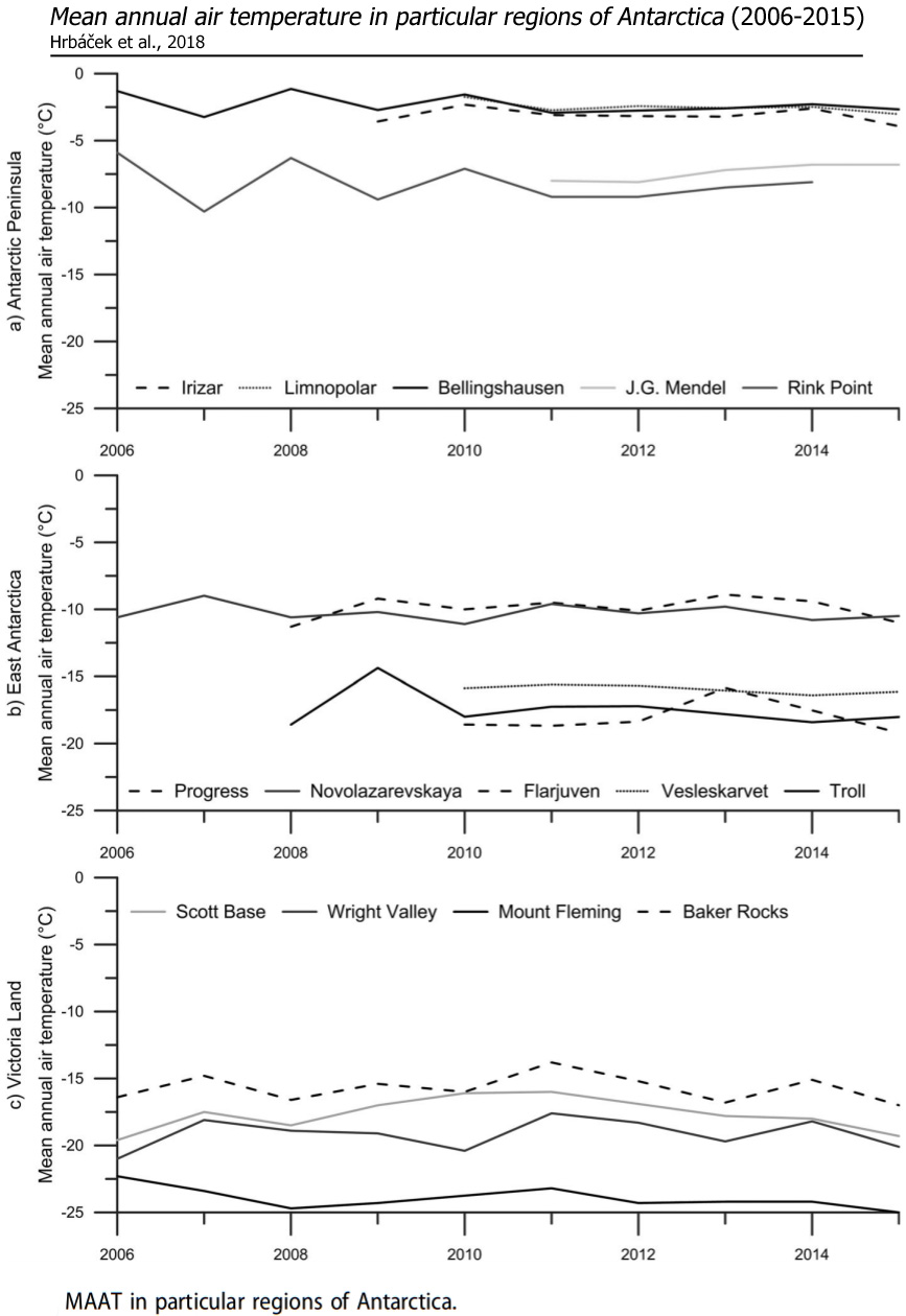
It is well documented in the scientific literature that climatic trends in and around Antarctica are predominantly controlled by natural mechanisms and internal variability, not greenhouse gas emissions.
A newly published paper (Scott, 2019), for example, identifies the forcing mechanisms behind the ice melt in the Amundsen Sea region of the WAIS during 1979-2017. Neither anthropogenic influences or greenhouse gas concentrations are mentioned anywhere in the paper as factors in Antarctic ice melt trends.
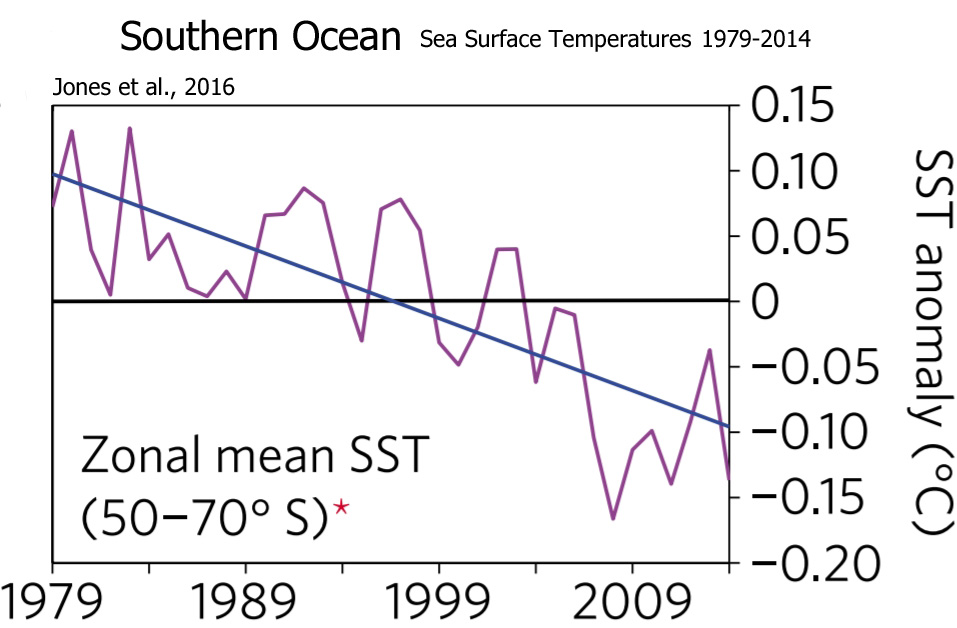
In a comprehensive analysis of the surface climate in and around Antarctica during 1979-2014 – including the cooling Southern Ocean – 25 scientists (Jones et al., 2016) assert that climate models predicated on anthropogenic forcing "are not compatible with the observed trends", and that "natural variability overwhelms the forced [anthropogenic] response in the observations".
Recent climate trends for the West Antarctic Ice Sheet have not offset the long-term cooling trend. The region was actually much warmer than modern for most of the last 2000 years.
In fact, recent paleoclimate evidence suggests (Stenni et al., 2017) that "no continent scale warming of Antarctica is evident in the last century."
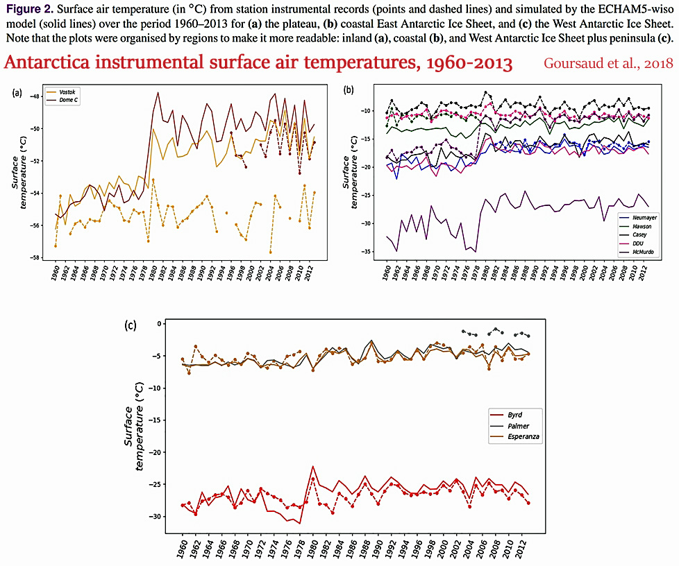
An earlier (2008) continent-wide climate data compilation revealed that although models of anthropogenic forcing simulated a climate warming of +0.75°C, Antarctica as a whole warmed by "only 0.2°C" over the last century.
Most of the continent has cooled since the early 1900s.
The Antarctic Peninsula, which warmed by "several degrees", drove the net continental temperature trend into positive territory, compensating for the cooling throughout East Antarctica.
As mentioned, the Antarctic Peninsula was the only anomalously warming sector of an otherwise-cooling Antarctic continent over the last several decades to century. It warmed by a rapid +0.32°C per decade from 1979-1997.
Then, beginning in about 1998-'99, the Peninsula began cooling even more rapidly than it had been warming. By 2014, all of the warming since 1979 had been offset, revealing an overall non-warming trend (Turner et al., 2016).
The northern-most portion of the Antarctic Peninsula cooled by -1.98°C between 2008-2014.
The Larsen Ice Shelf station has been cooling at a rate of -1.8°C per decade since 1995.
It is widely accepted that geothermal heat flux (volcanic activity) beneath the West Antarctic ice sheet – and Thwaites Glacier – is a "critical factor" in the active melting for the region.
Considering widespread modeling failures with trend simulation for Antarctica, perhaps there should be a reassessment of the factors and mechanisms underpinning the continent's variable climate and ice sheet melt.
The assumption that humans are driving the changes in Antarctica is not compatible with observations.
 Open Access
 This article is licensed under a Creative Commons Attribution-NonCommercial 3.0 Unported Licence.
 Open Access
 This article is licensed under a Creative Commons Attribution 3.0 Unported Licence.